Intro
In an earlier post I provided a template for creating a basic waterfall graph. Here I introduce a slightly more complex version with stacked bars over a time series. I use dplyr, ggplot2 and lubridate libraries.
Stacked Waterfall Graphs
This is a version of a waterfall graph I have found useful for showing delivery of commitments over time. The scenario is one where there are multiple groups with monthly deliverables. We want to see progress over time, current state, and timing of future deliverables through to end state or project completion.
I start by creating several months of mock data based on the current date. Each record is assumed to be one deliverable owned by a Group (G1, G2, G3) and due or already delivered during the Month (spanning two months prior and three months forward for the sake of illustration).
# Create mock data
month_range <- -2:3
df <- data.frame()

for (r in month_range){

    g1 <- sample(3:8,1)
    g2 <- sample(3:15,1)
    g3 <- sample(3:12,1)

    group <- data.frame(Group = c(rep("G1",g1), rep("G2", g2), rep("G3", g3)))
    month <- data.frame(Month = c(rep(floor_date(today() %m+% months(r), "month"), sum(g1, g2, g3))))
    set <- data.frame(Group = group, Month = month)
    df <- rbind(df, set)
}
The initial data set should look like this.
# Each record corresponds to a scheduled deliverable
rbind(head(df,5), tail(df,5))
## Group Month
## 1 G1 2019-04-01
## 2 G1 2019-04-01
## 3 G1 2019-04-01
## 4 G1 2019-04-01
## 5 G1 2019-04-01
## 102 G3 2019-09-01
## 103 G3 2019-09-01
## 104 G3 2019-09-01
## 105 G3 2019-09-01
## 106 G3 2019-09-01Once we have such a dataset in this format, the first step toward creating a waterfall graph is to define the starting values in the time series. To do this, I create a new variable Value and set it to -1 for each record. Then I create a new record for each Group that is the inverse of the sum of the Value field for the Group. I set the Month field for these new records to be the month prior to the first delivery month. The sum of the Value column should be zero.
df$Value <- -1

df2 <- df %>%
    select(Group, Value) %>%
    group_by(Group) %>%
    summarise(Value = sum(-Value)) %>%
    ungroup() %>%
    mutate(Month = floor_date(min(df$Month) %m+% (months(-1)))) %>%
    select(Group, Month, Value)

df <- rbind(df2,df)

df$Month <- ymd(df$Month)  #This date conversion is necessary for scale_x_date when we go to plot

all.equal(sum(df$Value), 0)   # check that the sum of the values is zero
## [1] TRUEThe data set should now look like this.
rbind(head(df,5), tail(df,5))## # A tibble: 10 x 3
## Group Month Value
## <fct> <date> <dbl>
## 1 G1 2019-03-01 26
## 2 G2 2019-03-01 38
## 3 G3 2019-03-01 42
## 4 G1 2019-04-01 -1
## 5 G1 2019-04-01 -1
## 6 G3 2019-09-01 -1
## 7 G3 2019-09-01 -1
## 8 G3 2019-09-01 -1
## 9 G3 2019-09-01 -1
## 10 G3 2019-09-01 -1Then we use the approach to generate min and max values I explained in my last post to generate the end and start values for x and y coordinates for each month.
data1 <- df %>%
    select(Month, Value) %>%
    group_by(Month) %>%
    summarise(Value = sum(Value)) %>%
    ungroup()

data1 <- data1  %>%
    mutate(
        yend = round(cumsum(Value), 3),
        ystart = lag(cumsum(Value), default = 0),
        xstart = c(head(Month, -1), NA),
        xend = c(tail(Month, -1), NA))
The data1 set will look something like this.
data1## # A tibble: 7 x 6
## Month Value yend ystart xstart xend
## <date> <dbl> <dbl> <dbl> <date> <date>
## 1 2019-03-01 106 106 0 2019-03-01 2019-04-01
## 2 2019-04-01 -12 94 106 2019-04-01 2019-05-01
## 3 2019-05-01 -19 75 94 2019-05-01 2019-06-01
## 4 2019-06-01 -21 54 75 2019-06-01 2019-07-01
## 5 2019-07-01 -15 39 54 2019-07-01 2019-08-01
## 6 2019-08-01 -17 22 39 2019-08-01 2019-09-01
## 7 2019-09-01 -22 0 22 NA NANext, we create another data set that captures the start and end values for x and y coordinates for each group per month. Then we join the data1 and data2 sets together by Month.
data2 <- df %>%
    select(Month, Group, Value) %>%
    group_by(Month, Group) %>%
    summarise(Value = sum(Value)) %>%
    ungroup()

data2 <- data2 %>%
    mutate(
       yend2 = cumsum(Value),
       ystart2 = lag(cumsum(Value), default = 0)
    )

data2 <- data2 %>%
    left_join(data1, by = "Month") %>%
    select(-c("Value.x", "Value.y"))  # These variables are no longer needed
The beginning and end of the data2 set will look like this.
rbind(head(data2,5), tail(data2,5))## # A tibble: 10 x 8
## Month Group yend2 ystart2 yend ystart xstart xend
## <date> <fct> <dbl> <dbl> <dbl> <dbl> <date> <date>
## 1 2019-03-01 G1 26 0 106 0 2019-03-01 2019-04-01
## 2 2019-03-01 G2 64 26 106 0 2019-03-01 2019-04-01
## 3 2019-03-01 G3 106 64 106 0 2019-03-01 2019-04-01
## 4 2019-04-01 G1 100 106 94 106 2019-04-01 2019-05-01
## 5 2019-04-01 G2 97 100 94 106 2019-04-01 2019-05-01
## 6 2019-08-01 G2 30 36 22 39 2019-08-01 2019-09-01
## 7 2019-08-01 G3 22 30 22 39 2019-08-01 2019-09-01
## 8 2019-09-01 G1 18 22 0 22 NA NA
## 9 2019-09-01 G2 9 18 0 22 NA NA
## 10 2019-09-01 G3 0 9 0 22 NA NAFinally, we are ready to graph. We start with a custom label for the x-axis. The first column that is going to appear on the graph will be the total of all of the deliverables and I will call this “Start Point” instead of giving it a month value. The following columns, the delivery months, I will label with the appropriate month descriptor. Note that because I set the scale of the x-axis to be months, I use +/- a number of days to control the width of the bars when using geom_rect().
month_label <- c("Start Point", tail(format(as.Date(seq(from = min(data1$Month), to = max(data1$Month),
                                                          by = "month")), "%b-%y"), -1))

ggplot(data2) +
    geom_rect(aes(xmin = ymd(Month) - days(12),
                  xmax = ymd(Month) + days(12), ymin = yend2, ymax = ystart2,
                  fill = Group),
              colour = "black") +
    geom_segment(data = data1[1:(nrow(data1) -1),],aes(x = ymd(xstart),
                                                       xend = ymd(xend),
                                                       y = yend,
                                                       yend = yend)) +
    geom_hline(yintercept = 0, linetype=2) +
    geom_vline(xintercept = floor_date(today(), "month"), linetype=1, colour = "red",
               show.legend = TRUE) +
    annotate("text", x = floor_date(today(), "month"), y = -3, label = "Current Month", size = 3) +
    labs(y = "Number of Deliverables", x = "Delivery Timeframe",
         title = "Waterfall Schedule of Deliverables") +
    scale_x_date(breaks = seq(from = min(data1$Month), to = max(data1$Month), by = "month"), labels = month_label) +
    theme_bw()+
    theme(legend.position = "right", panel.grid = element_blank(), axis.text.x = element_text(angle = 90, vjust = .5))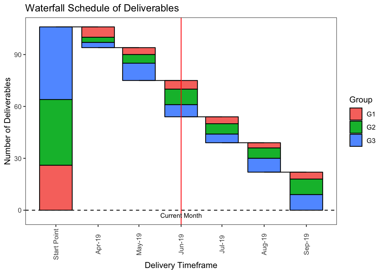
Here we have generated a waterfall graph that shows the schedule of monthly deliverables for several groups as stacked bars over a time based x-axis. We start with the full set of deliverables on the left and as we move to the right, show actual deliveries up to the Current Month and the schedule of future deliverables through to completion.